This post provides Stata commands to create a panel dataset out of the College Scorecard data. The first steps take only a few minutes, then the final destring step takes quite a while to run (at least an hour).
Step 1: Download the .csv files from here
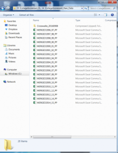
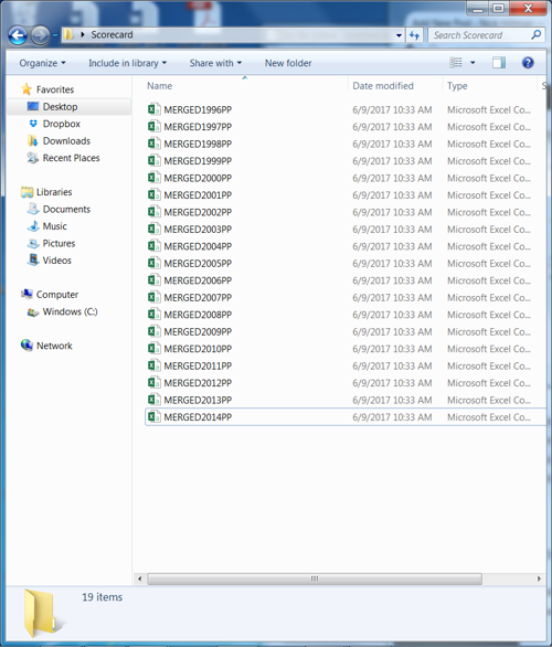
In this example, I download these files into a “Scorecard” folder located on my desktop.
Notice how the file names have underscores in them. The first file is titled “MERGED1996_97_PP” and so on. Let’s drop the underscore and number in between (“_97_”) so the file now is titled “MERGED1996PP” and do this for each file:

Step 2: Convert .csv files to .dta files
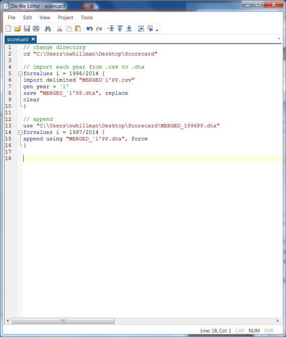
Our raw data is now downloaded and prepped. Open a Stata .do file and import these .csv files. The following loop is a nice way to do this efficiently:
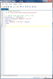
- Row 2 tells Stata where to find the raw .csv data.
- Row 5 tells Stata to remember (as “i”) any number that fall between 1996 and 2014.
- Row 6 tells Stata to import any .csv file in my directory named “MERGED`i’PP” — here the `i’ is replaced by the numbers 1996 through 2014. This is why we got rid of the underscores in Step 1, it helps this loop operate efficiently.
- Row 7 generates a new variable called “year” and sets its value equal to the corresponding year in the file.
- Row 8 saves each .csv file as a .dta file and keeps the same file naming convention as before.
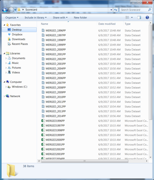
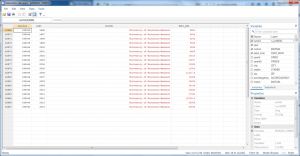
- Row 9 tells Stata to start anew after each year so we end up with the following files in our directory:
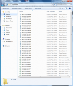
Notice the .dta files are all now here and named in the exact same way as the original .csv files (well, technically I added an underscore after “MERGED”). This loop takes a few minutes to run.
Step 3: Append each year into a single file
Now that we have individual files, we want to stack them all on top of each other. We have to start somewhere, so let’s open the 1996 .dta file and then append all future years, 1997 through 2014, onto this file:

We will do this in a small loop this time, where:
- Row 13 tells Stata to open the 1996 .dta file
- Row 14 tells Stata to remember as “i” the numbers 1997 to 2014
- Row 15 tells Stata to append onto the 1996 file each .dta that corresponds with the year `i’. The “force” command is needed here only because some years a variable is coded as a string and others numeric, so this just tells Stata to bypass that quirk.
Step 4: Destring the data
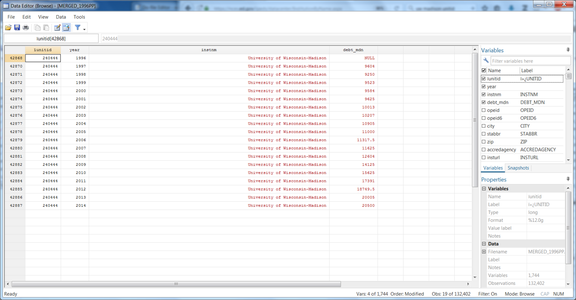
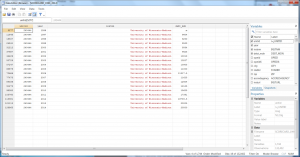
The data is now in a panel format, where each row contains a unique institution and year. Let’s take a quick look at UW-Madison (unitid=240444) by using the following command:
br ïunitid year instnm debt_mdn if ïunitid==240444
We’re almost done, but notice a couple of quirks here. First, the median debt value is red, meaning it is string (because 1996 is “NULL”). Second, the variable ïunitid should be renamed to just plain old “unitid” – otherwise, things look pretty good here in terms of setting up a panel.
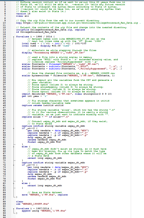
The following loop will clean this all up for us. It took me at least an hour, be warned. (Thank you Nick Cox for your helpful de-bugging!)
- Row 19 renames ïunitid to unitid
- Row 20 tells Stata to find string variables
- Row 21 tells Stata to remember as “x” all variables in the file
- Rows 22 and 23 replace all those NULLs and PrivacySuppressed cells with “.n” and “.p” missing values, respectively.
- Row 25 destrings and replaces all variables
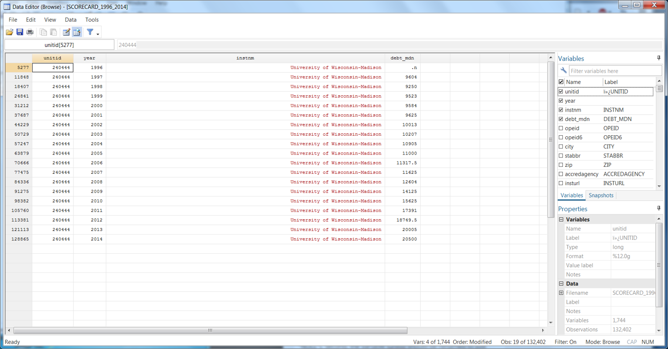
So now when we look at UW-Madison, we see the median debt values are black, meaning they are destringed (destrung?) with the “NULL” value for 1996 missing.
Step 5: Add variable and value labels
Thanks to Kevin Fosnacht (Indiana University), you can also add labels with the commands found below in the .do file. Thanks, Kevin!
Step 6: Save the new file so you don’t have to run all this again.
You now have all Scorecard data from 1996 to 2014 in a single panel dataset, allowing you to merge with other data sources and analyze this with panel data techniques.
There are several other ways one could go about managing this dataset and creating the panel, so forgive me for any omissions or oversights here. My goal is to simply help remove a data access barrier to facilitate greater research use of this public resource. Grad students developing their research programs might find this a useful data source for contributing to and extending higher education policy scholarship.
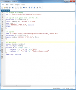
.do file: scorecard
Update 6/12/2017: the “.n” and “.p” command had a small bug on the destring loop. But thanks to Nick Cox, this is now fixed! Also, Kevin Fosnacht was so kind as to share his relabeling code, many thanks!